VTK Book Figure Examples
The Visualization Toolkit Text Book was first published in 1995. At that time, the book was unique. It presented the theory behind computer graphics and visualization algorithms. It also provided a free C++ toolkit called VTK. Each theory chapter of the book wrapped up with a section called Putting It All Together. These sections provided examples using the VTK software. The examples were written in C++ or Tcl. As VTK matured, the Application Programming Interface (API) also matured. For example, today, C++ and Python are the preferred languages, although Java is still available. Tcl is no longer supported. Although the VTK software has always been free, until recently the VTK Book was only available commercially. Now, the book, like the software, is also free. View or download the book here.
Even though the book is over 20 years old, the concepts in the book are still relevant. The dozens of examples in the book are also still valuable for learning and using VTK. We have begun an effort to convert all of the examples in the book into C++ and present them Chapter by Chapter. These examples supplement the hundreds of examples on the VTK Examples web site.
Since some of the API's have changed, the new implementations may differ from those in the book. Also, since Tcl used less frequently, the examples have been converted to C++. The examples are also enhanced by newer VTK features, like vtkNamedColors and vtkSmartPointer.
Each Figure example
-
links to the source code of the new implementation,
-
links to the doxygen documentation for classes demonstrated,
-
shows the original figure caption and,
-
if the example produces an image, links to the full resolution image. If the caption includes a source file reference, e.g. bluntStr.cxx or rotations.tcl, that reference links to the original source code.
-
if there is a corresponding Python example, a link to that example follows the figure line.
Please enjoy this new effort to revive and maintain the VTK Figure examples.
Chapter 3 - Computer Graphics
| Figure | Caption | Image |
|---|---|---|
| Figure 3-7 | Flat and Gouraud shading. Different shading methods can dramatically improve the look of an object represented with polygons. On the top, flat shading uses a constant surface normal across each polygon. On the bottom, Gouraud shading interpolates normals from polygon vertices to give a smoother look. | 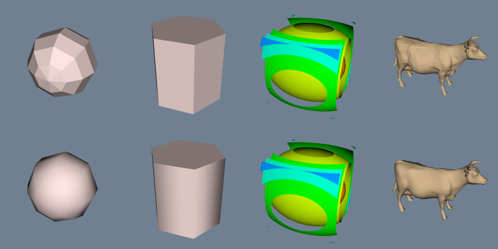 |
| Figure 3-10 | Effects of specular coefficients. Specular coefficients control the apparent “shininess” of objects. The top row has a specular intensity value of 0.5; the bottom row 1.0. Along the horizontal direction the specular power changes. The values (from left to right) are 5, 10, 20, and 40 (SpecularSpheres.cxx). |  |
| Figure 3-12 | Camera movements around focal point (camera.tcl). |  |
| Figure 3-13 | Camera movements centered at camera position (camera2.tcl). |  |
| Figure 3-24 | Illustrative diagram of graphics objects (Model.cxx). | 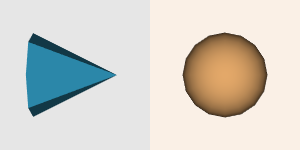 |
| Figure 3-26 | Examples of source objects that procedurally generate polygonal models. These nine images represent just some of the capability of VTK. From upper left in reading order: sphere, cone, cylinder, cube, plane, text, random point cloud, disk (with or without hole), and line source. Other polygonal source objects are available; check subclasses of vtkPolyDataAlgorithm. |  |
| Figure 3-27 | Four frames of output from Cone3.cxx. | 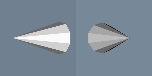 |
| Figure 3-28 | Modifying properties and transformation matrix (Cone4.cxx) |  |
| Figure 3-31 | Rotations of a cow about her axes. In this model, the x axis is from the left to right; the y axis is from bottom to top; and the z axis emerges from the image. The camera location is the same in this and the following four images (rotations.tcl). |  |
| Figure 3-31a | Perform six rotations of a cow about her x-axis. |  |
| Figure 3-31b | Perform six rotations of a cow about her y-axis. | 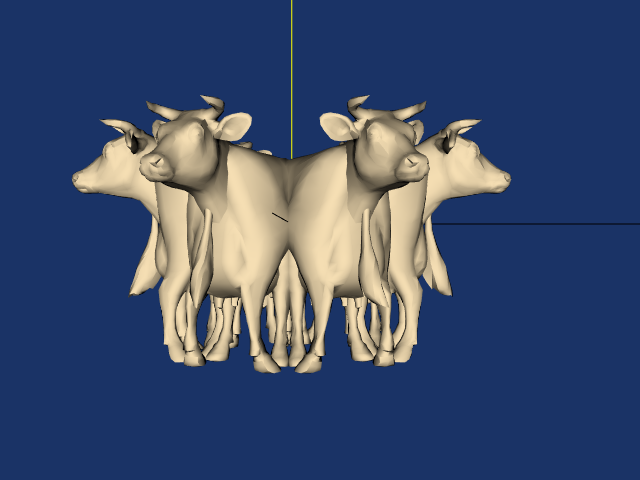 |
| Figure 3-31c | Perform six rotations of a cow about her z-axis. |  |
| Figure 3-31d | First a rotation of a cow about her x-axis, then six rotations about her y-axis. |  |
| Figure 3-32 | The cow "walking" around the global origin (walkCow.tcl). |  |
| Figure 3-33a | The cow rotating about a vector passing through her nose. (a) With origin (0,0,0). (walkCow.tcl). |  |
| Figure 3-33b | The cow rotating about a vector passing through her nose. (b) With origin at (6.1,1.3,.02). (walkCow.tcl). |  |
Chapter 4 - The Visualization Pipeline
| Figure | Caption | Image |
|---|---|---|
| Figure 4–1 | Visualizing a quadric function (Sample.cxx) |  |
| Figure 4-13 | Importing and exporting files in VTK. An importer creates a vtkRenderWindow that describes the scene. Exporters use an instance of vtkRenderWindow to obtain a description of the scene (3dsToRIB.tcl) and (flamingo.tcl). | 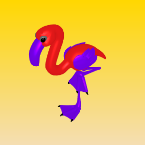 |
| Figure 4-19 | A simple sphere (ColorSph.cxx). |  |
| Figure 4-20 | The addition of a transform filter to the previous example. (StrSph.cxx). | |
| Figure 4-21 | An example of multiple inputs and outputs (Mace.cxx). | 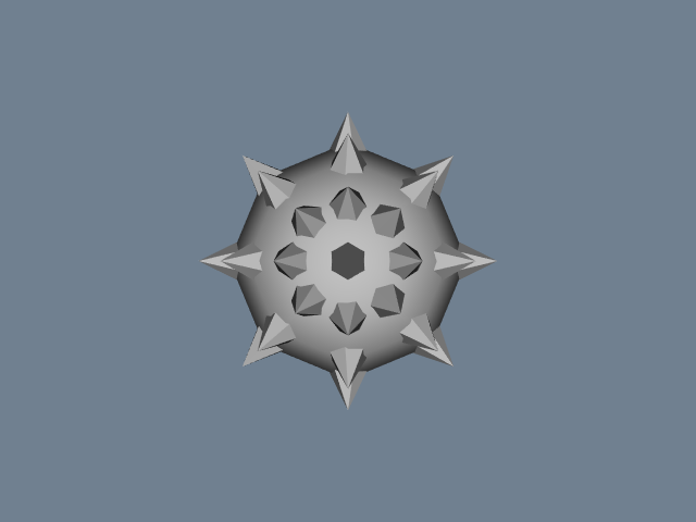 |
| Figure 4-22 | A network with a loop. VTK 5.0 does not allow you to execute a looping visualization network; this was possible in previous versions of VTK. (LoopShrk.cxx). | 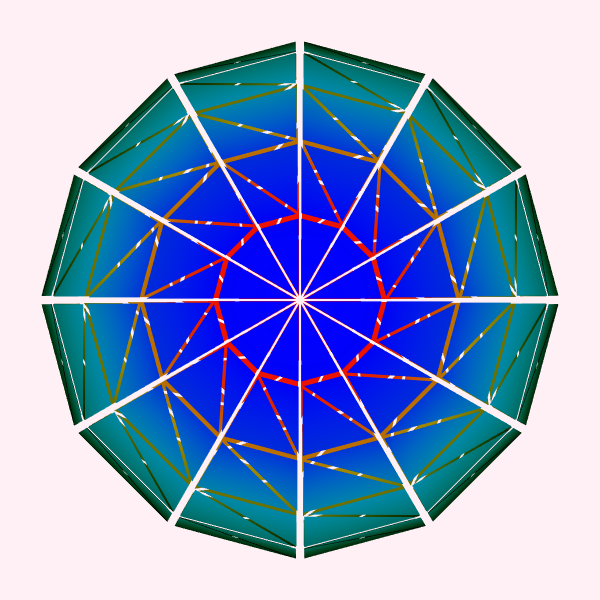 |
Chapter 5 - Basic Data Representation
| Figure | Caption | Image |
|---|---|---|
| Figure 5-17 | Creation of polygonal cube (Cube.cxx). | 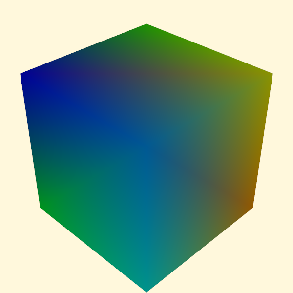 |
| Figure 5-18 | Creating a image data dataset. Scalar data is generated from the equation for a sphere. Volume dimensions are 26 x 26 x 26 (Vol.cxx). |  |
| Figure 5-19 | Creating a structured grid dataset of a semi-cylinder. Vectors are created whose magnitude is proportional to radius and oriented in tangential direction (SGrid.cxx). | 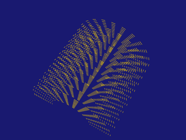 |
| Figure 5-20 | Creating a rectilinear grid dataset. The coordinates along each axis are defined using an instance of vtkDataArray (RGrid.cxx). |  |
| Figure 5-21 | Creation of an unstructured grid (UGrid.cxx). |  |
Chapter 6 - Fundamental Algorithms
| Figure | Caption | Image |
|---|---|---|
| Figure 6-6 | Marching cubes cases for 3D isosurface generation. The 256 possible cases have been reduced to 15 cases using symmetry. Dark vertices are greater than the selected isosurface value. | 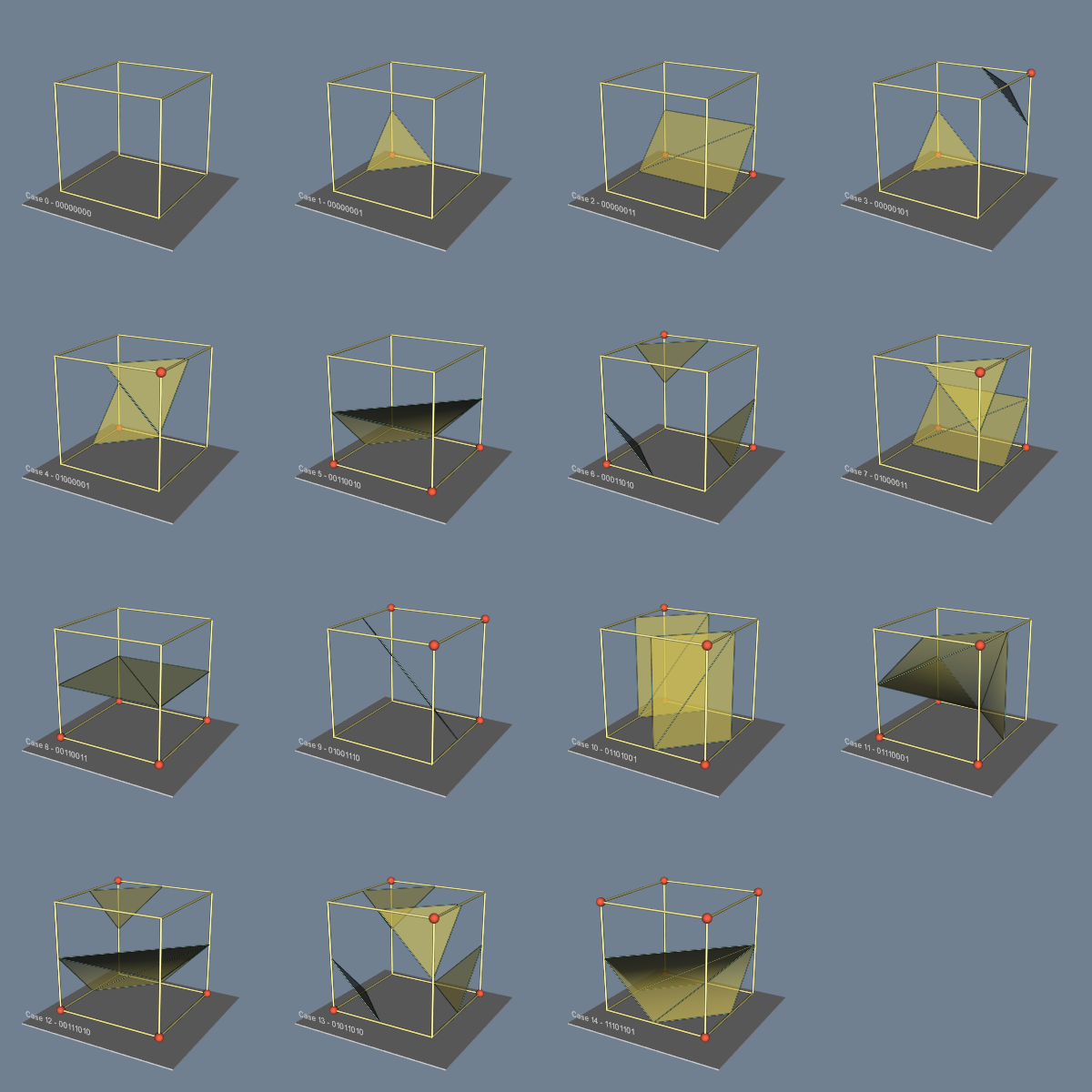 |
| Figure 6-9a | Marching cubes, case 3 is rotated 90 degrees about the y-axis with no label. |  |
| Figure 6-9b | Marching cubes, case 7 is rotated 180 degrees about the y-axis with no label. | 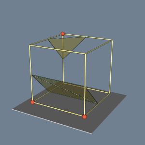 |
| Figure 6-10 | Marching cubes complementary cases. Cases 3c, 6c, 7c, 10c, 12c and 13c are displayed. |  |
| Figure 6-11a | Contouring examples. (a) Marching squares used to generate contour lines (headSlic.tcl). Also see FlyingHeadSlice (cxx) and FlyingHeadSlice (Python) | 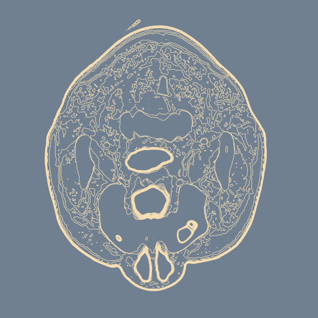 |
| Figure 6-11b | Contouring examples. (b) Marching cubes surface of human bone (headBone.tcl). | 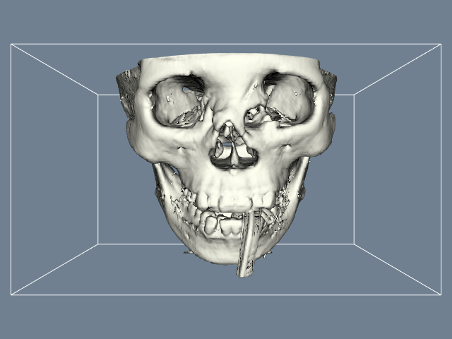 |
| Figure 6-11c | Contouring examples. (c) Marching cubes surface of flow density (combIso.tcl). | 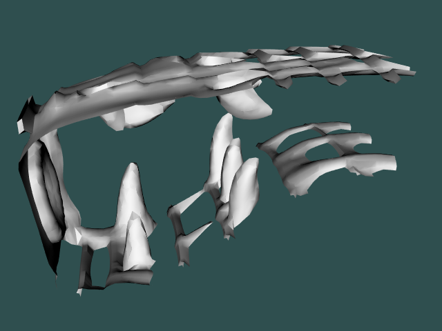 |
| Figure 6-11d | Contouring examples. (d) Marching cubes surface of iron-protein (ironPIso.tcl). | 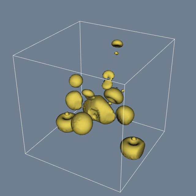 |
| Figure 6-12 | Computing scalars using normalized dot product. Bottom half of figure illustrates technique applied to terrain data from Honolulu, Hawaii (hawaii.tcl). |  |
| Figure 6-13 | Vector visualization techniques: (a) oriented lines; (b) using oriented glyphs; (c) complex vector visualization (complexV.tcl). | 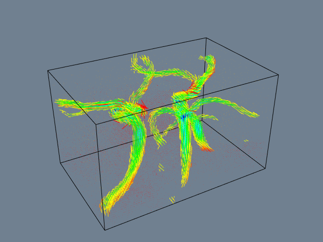 |
| Figure 6-14a | Warping geometry to show vector field: (a) Beam displacement (vib.tcl). | 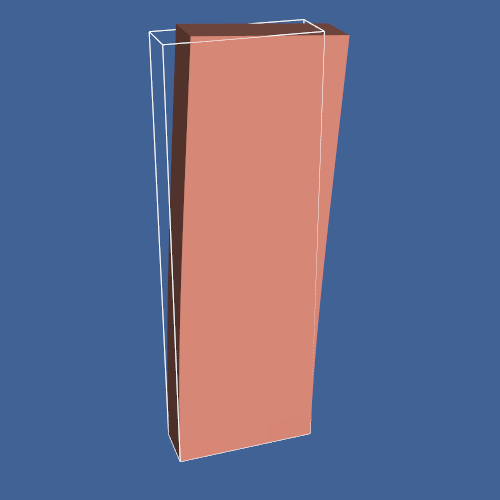 |
| Figure 6-14b | Warping geometry to show vector field: (b) Flow momentum (velProf.tcl). | 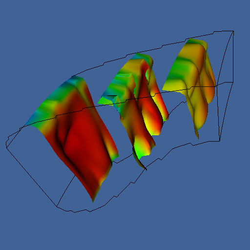 |
| Figure 6-15b | Vector displacement plots. (b) Surface plot of vibrating plate. Dark areas show nodal lines. Bright areas show maximum motion (dispPlot.tcl). |  |
| Figure 6-18 | Flow velocity computed for a small kitchen (top and side view). Forty streamlines start along the rake positioned under the window. Some eventually travel over the hot stove and are convected upwards (Kitchen.cxx). | 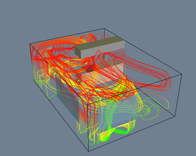 |
| Figure 6-19 | Dashed streamlines around a blunt fin. Each dash is a constant time increment. Fast moving particles create longer dashes than slower moving particles. The streamlines also are colored by flow density scalar (bluntStr.cxx). | 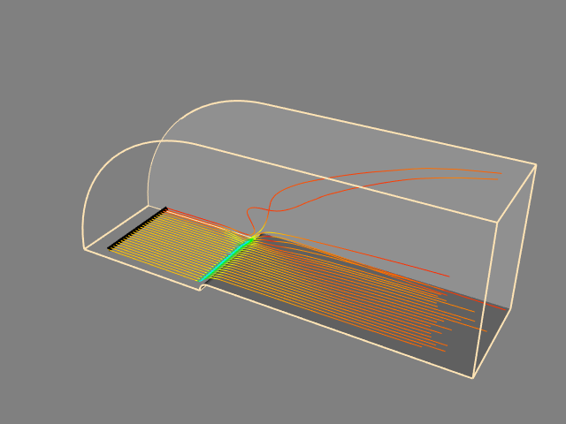 |
| Figure 6-22a | Tensor visualization techniques; (a) Tensor axes TenAxes.tcl |  |
| Figure 6-22b | Tensor visualization techniques; (b) Tensor ellipsoids TenEllip.tcl | 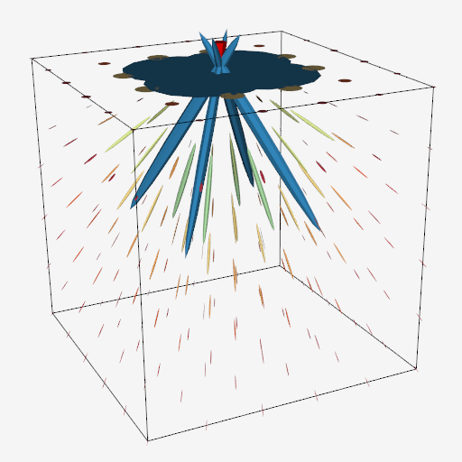 |
| Figure 6-23b | Sampling functions: (b) Isosurface of sampled sphere (sphere.tcl). |  |
| Figure 6-23c | Sampling functions: (b) Isosurface of sampled sphere; (c) Boolean combination of two spheres, a cone, and two planes. (One sphere intersects the other, the planes clip the cone.) (iceCream.tcl). |  |
| Figure 6-24b | Implicit functions used to select data: (b) Two ellipsoids combined using the union operation used to select voxels from a volume. Voxels shrunk 50 percent (extractD.tcl). | 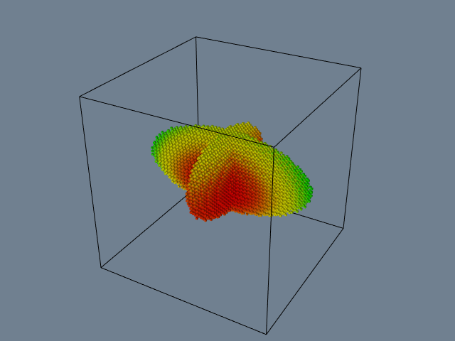 |
| Figure 6-25 | Visualizing a Lorenz strange attractor by integrating the Lorenz equations in a volume. The number of visits in each voxel is recorded as a scalar function. The surface is extracted via marching cubes using a visit value of 50. The number of integration steps is 10 million, in a volume of dimensions 200 3 . The surface roughness is caused by the discrete nature of the evaluation function (Lorenz.cxx) | 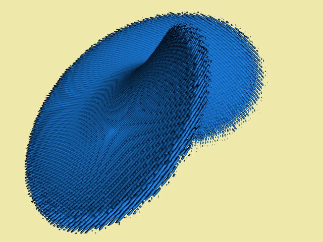 |
| Figure 6-28 | Implicit modelling used to thicken a stroked font. Original lines can be seen within the translucent implicit surface ((hello.tcl). |  |
| Figure 6-3 | Flow density colored with different lookup tables. Top-left: grayscale; Top-right rainbow (blue to red); lower-left rainbow (red to blue); lower-right large contrast (rainbow.tcl). | 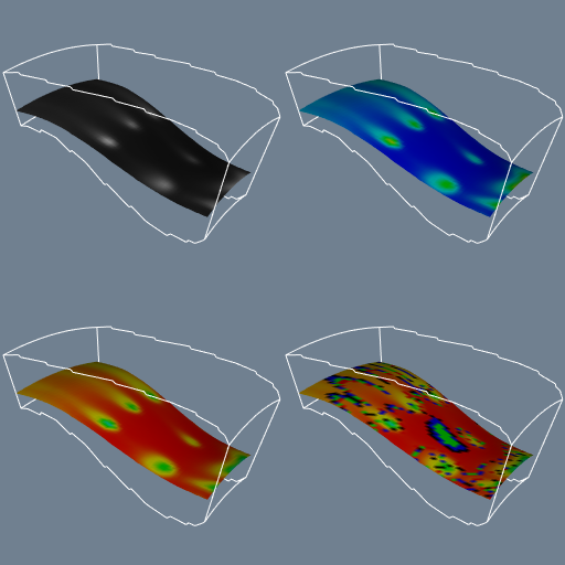 |
| Figure 6-30 | Glyphs indicate surface normals on model of human face. Glyph positions are randomly selected (spikeF.tcl). |  |
| Figure 6-31 | Cut through structured grid with plane. The cut plane is shown solid shaded. A computational plane of constant k value is shown in wireframe for comparison (cut.tcl). The colors correspond to flow density. Cutting surfaces are not necessarily planes: implicit functions such as spheres, cylinders, and quadrics can also be used. |  |
| Figure 6-32 | 100 cut planes with opacity of 0.05. Rendered back-to-front to simulate volume rendering (PseudoVolumeRendering.tcl). | 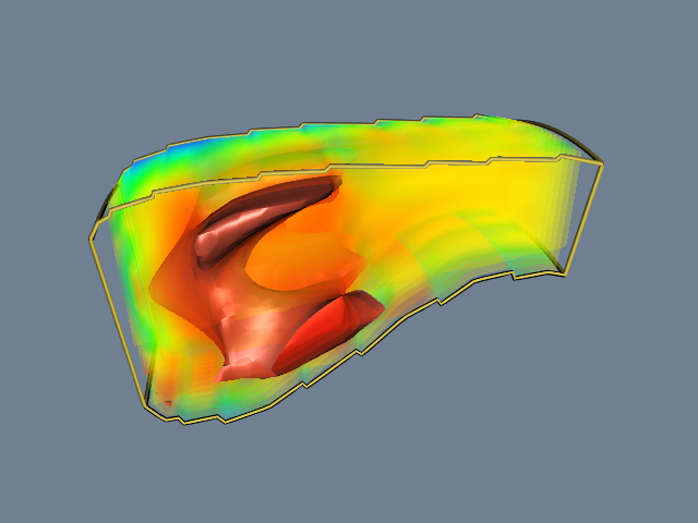 |
| Figure 6-33 | Cutting a surface model of the skin with a series of planes produces contour lines (cutModel.tcl). Lines are wrapped with tubes for visual clarity. | 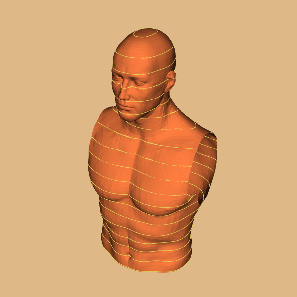 |
| Figure 6-39 | Contouring quadric function. Pipeline topology, C++ code, and resulting image are shown (contQuad.cxx). | 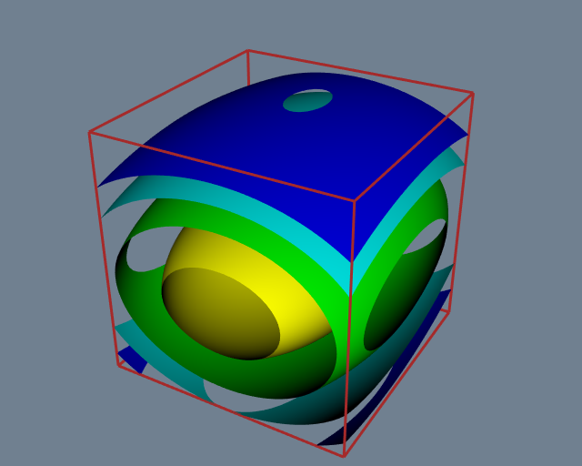 |
| Figure 6-43 | Visualizing blood flow in human carotid arteries. Cone glyphs indicate flow direction and magnitude. The code fragment shown is from the Tcl script thrshldV.tcl and shows creation of vector glyphs. |  |
| Figure 6-44 | Visualizing blood flow in the human carotid arteries. Streamtubes of flow vectors (streamV.tcl). | 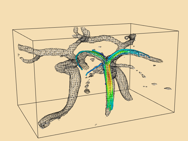 |
Chapter 7 - Advanced Computer Graphics
| Figure | Caption | Image |
|---|---|---|
| Figure 7-3 | One frame from a vector field animation using texture maps (animVectors.tcl). |  |
| Figure 7-33 | Example of texture mapping (TPlane.tcl). |  |
| Figure 7-34 | Volume rendering of a high potential iron protein (SimpleRayCast.tcl). | 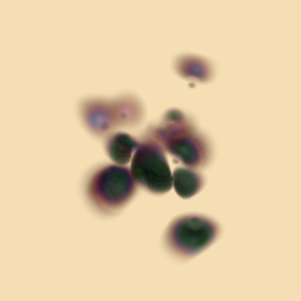 |
| Figure 7-36 | Example of motion blur (MotBlur.cxx). | 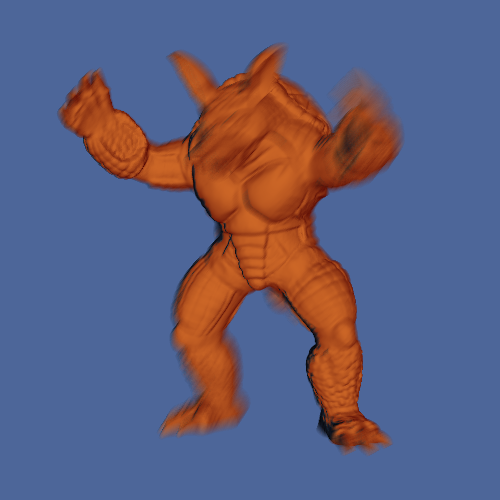 |
| Figure 7-37 | Example of a scene rendered with focal depth (CamBlur.cxx). | 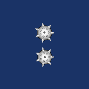 |
| Figure 7-39 | Using the vtkLineWidget to produce streamlines in the combustor dataset. The StartInteractionEvent turns the visibility of the streamlines on; the InteractionEvent causes the streamlines to regenerate themselves (LineWidget.tcl). | 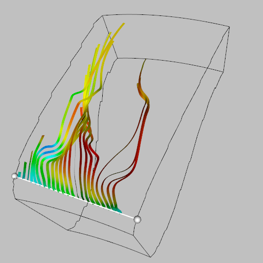 |
Chapter 8 - Advanced Data Representation
| Figure | Caption | Image |
|---|---|---|
| Figure 8-41a | (a) Linearly extruded fonts to show letter frequency in text (alphaFreq.cxx). | 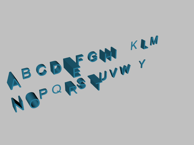 |
| Figure 8-41b | (b) Rotationally symmetric objects(bottle.tcl). | 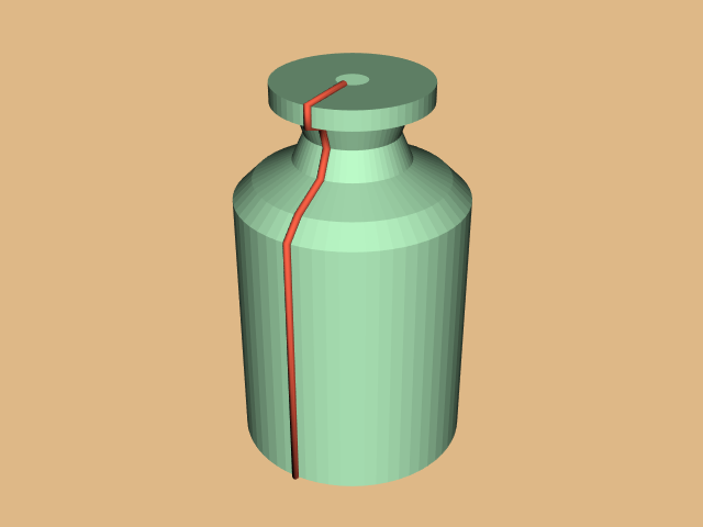 |
| Figure 8-41c | (c) Rotation in combination with linear displacement and radius variation (spring.tcl). |  |
Chapter 9 - Advanced Algorithms
| Figure | Caption | Image |
|---|---|---|
| Figure 9-4a | Carpet plots. (a) Visualization of an exponential cosine function. Function values are indicated by surface displacement. Colors indicate derivative values (expCos.cxx). |  |
| Figure 9-4b | Carpet plots. (b) Carpet plot of combustor flow energy in a structured grid. Colors and plane displacement represent energy values (warpComb.tcl). | 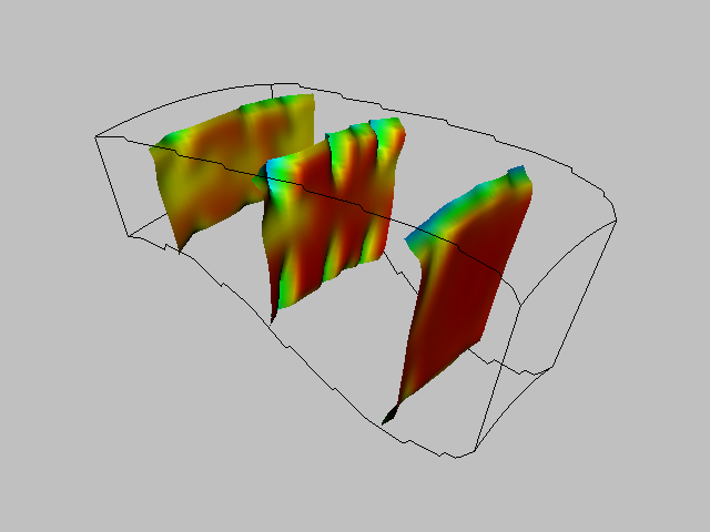 |
| Figure 9-10 | A scanned image clipped with a scalar value of 1/2 its maximum intensity produces a mixture of quadrilaterals and triangles (createBFont.tcl). |  |
| Figure 9-12d | The stream polygon. (d) Sweeping polygon to form tube (officeTube.tcl) . |  |
| Figure 9-15 | Example of hyperstreamlines (Hyper.tcl). The four hyperstreamlines shown are integrated along the minor principle stress axis. A plane (colored with a different lookup table) is also shown. | 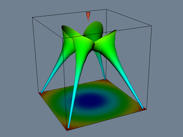 |
| Figure 9-19 | Probing data in a combustor. Probes are regular arrays of 50 by 50 points that are then passed through a contouring filter (probeComb.tcl). | 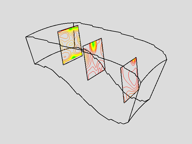 |
| Figure 9-21 | Triangle strip examples. (a) Structured triangle mesh consisting of 134 strips each of 390 triangles (stripF.tcl). (b) Unstructured triangle mesh consisting of 2227 strips of average length 3.94, longest strip 101 triangles. Images are generated by displaying every other triangle strip (uStripeF.tcl). |  |
| Figure 9-24 | Surface normal generation. (a) Faceted model without normals. (b)Polygons must be consistently oriented to accurately compute normals. (c)Sharp edges are poorly represented using shared normals as shown on the corners of this model. (d) Normal generation with sharp edges split (Normals.cxx). | 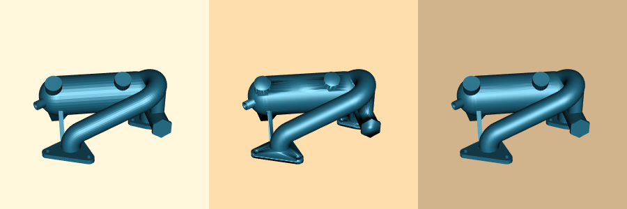 |
| Figure 9-27a | Examples of decimation algorithm. (a) Decimation of laser digitizer data (deciFran.tcl). |  |
| Figure 9-27b | Examples of decimation algorithm. (b) Decimation of terrain data (deciHawa.tcl). | 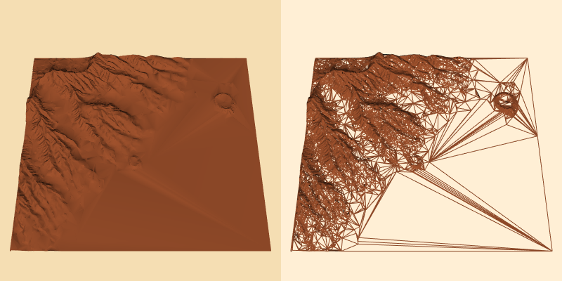 |
| Figure 9-38a | Elliptical splatting. (a) Single elliptical splat with eccentricity E=10. Cone shows orientation of vector (singleSplat.cxx). |  |
| Figure 9-38b | Elliptical splatting. (b) Surface reconstructed using elliptical splats into 100 3 volume followed by isosurface extraction. Points regularly subsampled and overlaid on original mesh (splatFace.tcl). |  |
| Figure 9-43a | Examples of texture thresholding. (a) Using scalar threshold to show values of flow density on planes for various values (texThresh.tcl). |  |
| Figure 9-43b | Examples of texture thresholding. (b) Boolean combination of two planes to cut nested spheres (tcutSph.cxx). | 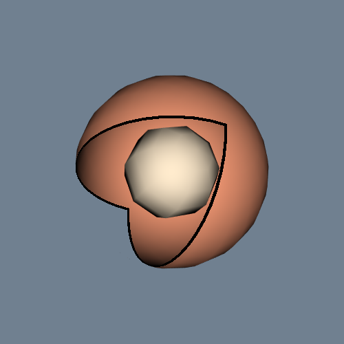 |
| Figure 9-45b | (b) Sixteen boolean textures applied to sphere (quadricCut.cxx). | 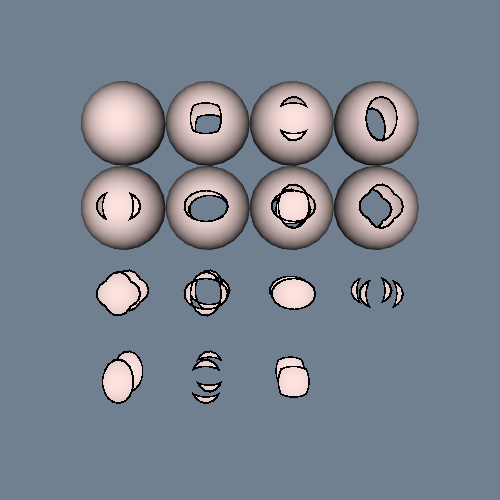 |
| Figure 9-47a | Using random point seeds to create streamlines (office.tcl). | 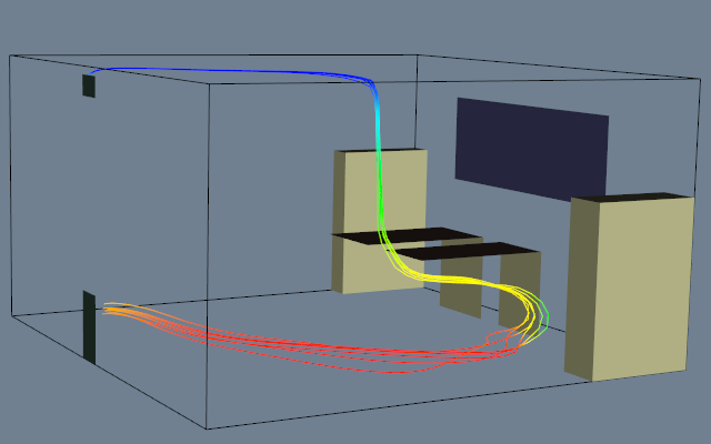 |
| Figure 9-47b | Using random point seeds to create streamlines (office.tcl). |  |
| Figure 9-48 | A plane clipped with a sphere and an ellipse. The two transforms place each implicit function into the appropriate position. Two outputs are generated by the clipper. (clipSphCyl.tcl). | 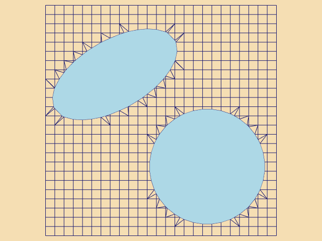 |
| Figure 9-50 | Visualization of multidimensional financial data. (finance.cxx). The gray/wireframe surface represents the total data population. The red surface represents data points delinquent on loan payment. |  |
| Figure 9-51a | The isosurface, with no connectivity filter applied connPineRoot.tcl. Data is from 256^3 volume data of the root system of a pine tree. | 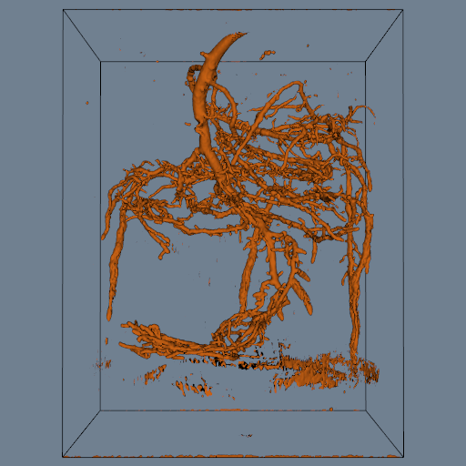 |
| Figure 9-51b | The isosurface after applying the connectivity filter to remove noisy isosurfaces connPineRoot.tcl. Data is from 256^3 volume data of the root system of a pine tree. |  |
| Figure 9-52a | The isosurface after applying the connectivity filter to remove noisy isosurfaces and reduce data size connPineRoot.tcl. Data is from 256^3 volume data of the root system of a pine tree. | |
| Figure 9-52b | The isosurface after applying the decimation and connectivity filters to remove noisy isosurfaces and reduce data size deciPineRoot.tcl. Data is from 256^3 volume data of the root system of a pine tree. | 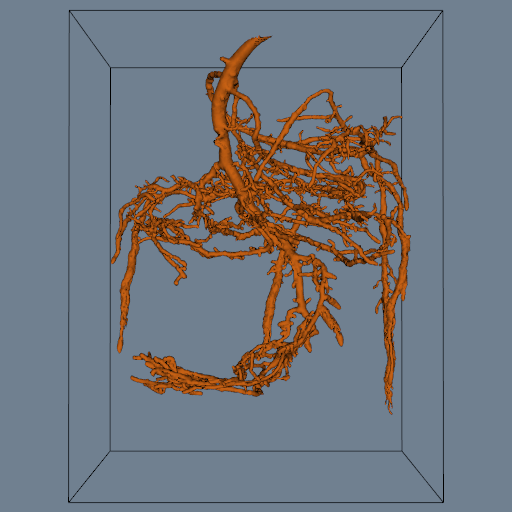 |
| Figure 9-53 | Texture cut used to reveal internal structure of a motor. Two cut planes are used in combination with transparent texture (motor.tcl). | 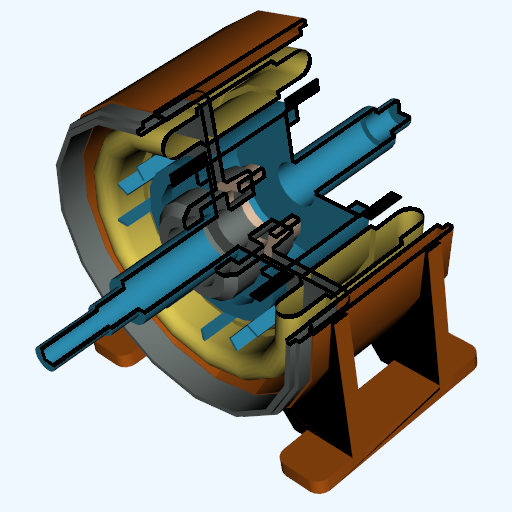 |
| Figure 9-54 | Two-dimensional Delaunay triangulation of a random set of points. Points and edges are shown highlighted with sphere glyphs and tubes (DelMesh.tcl) . Only the pipeline to generate triangulation is shown. |  |
Chapter 10 - Image Processing
| Figure | Caption | Image |
|---|---|---|
| Figure 10-3 | Comparison of Gaussian and Median smoothing for reducing low-probability high-amplitude noise (MedianComparison..tcl) |  |
| Figure 10-4 | Comparison of median and hybrid-median filters. The hybrid filter preserves corners and thin lines, better than the median filter. hybrid median (HybridMedianComparison.tcl. | 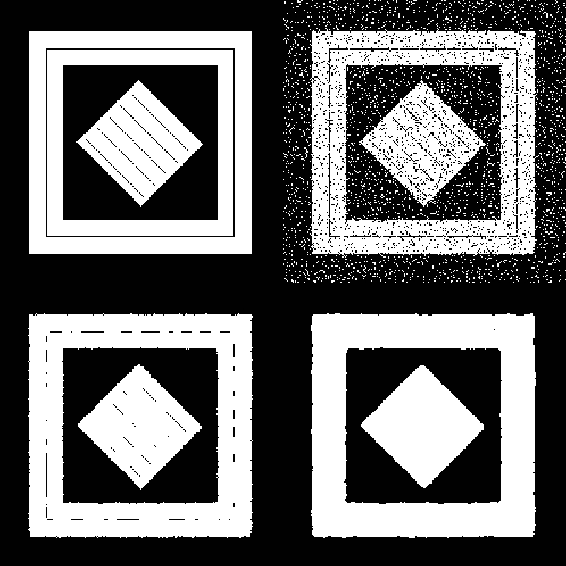 |
| Figure 10-5 | This figure demonstrates aliasing that occurs when a high-frequency signal is subsampled. High frequencies appear as low frequency artifacts. The lower left image is an isosurface of a skull after subsampling. The right image used a low-pass filter before subsampling to reduce aliasing (IsoSubsample.tcl). | 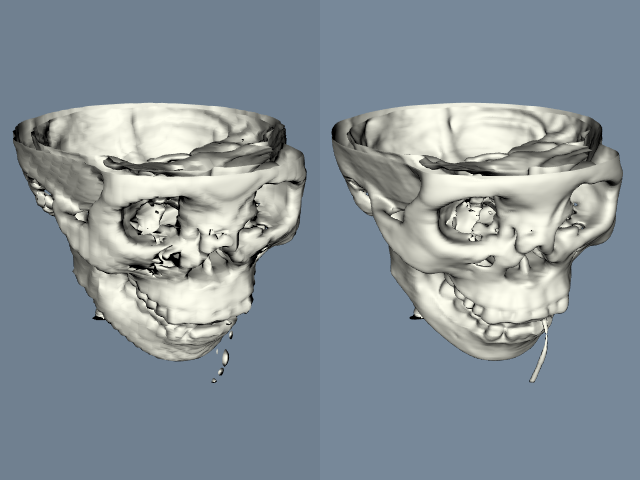 |
| Figure 10-6 | This MRI image illustrates attenuation that can occur due to sensor position. The artifact is removed by dividing by the attenuation profile determined manually. (Attenuation.tcl).. |  |
| Figure 10-9 | High-pass filters can extract and enhance edges in an image. Subtraction of the Laplacian (middle) from the original image (left) results in edge enhancement or a sharpening operation (right) (EnhanceEdges.tcl). | 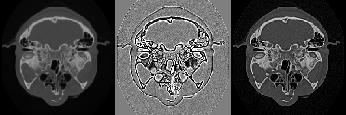 |
| Figure 10-10 | The discrete Fourier transform changes an image from the spatial domain into the frequency domain, where each pixel represents a sinusoidal function. This figure show an image and its power spectrum displayed using a logarithmic transfer function (VTKSpectrum.tcl). |  |
| Figure 10-11 | This figure shows two high-pass filters in the frequency domain. The Butterworth high-pass filter has a gradual attenuation that avoids ringing produced by the ideal high-pass filter with an abrupt transition (IdealHighPass.tcl). |  |
| Figure 10-12 | Convolution in frequency space treats the image as a periodic function. A large kernel can pick up features from both sides of the image. The lower-left image has been padded with zeros to eliminate wraparound during convolution. On the right, mirror padding has been used to remove artificial edges introduced by borders (Pad.tcl). | 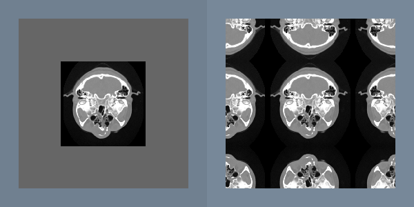 |
| Figure 10-14 | This figure demonstrates various binary filters that can alter the shape of segmented regions (MorphComparison.tcl). | 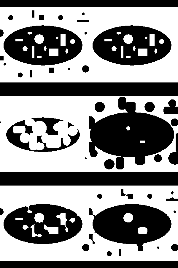 |
| Figure 10-16 | An imaging pipeline to visualize gradient information. The gradient direction is mapped into color hue value while the gradient magnitude is mapped into the color saturation (ImageGradient.tcl). | 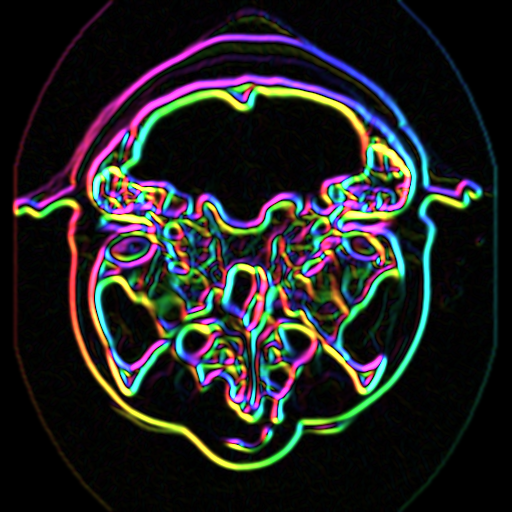 |
| Figure 10-17 | Combining the imaging and visualization pipelines to deform an image in the z-direction (imageWarp.tcl). The vtkMergeFilter is used to combine the warped surface with the original color data. | 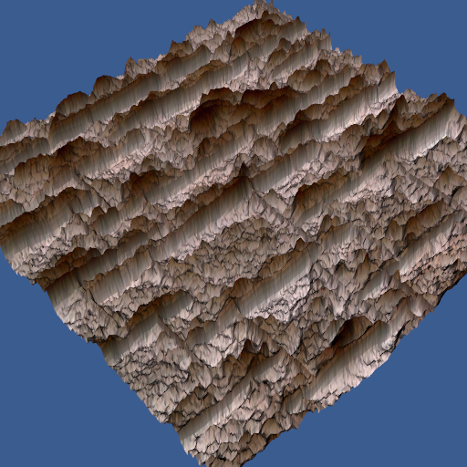 |
| Figure 10-2 | Low-pass filters can be implemented as convolution with a Gaussian kernel. (GaussianSmooth.tcl). |  |
Chapter 12 - Applications
| Figure | Caption | Image |
|---|---|---|
| Figure 12-2 | The skin extracted from a CT dataset of the head (Medical1.cxx). | 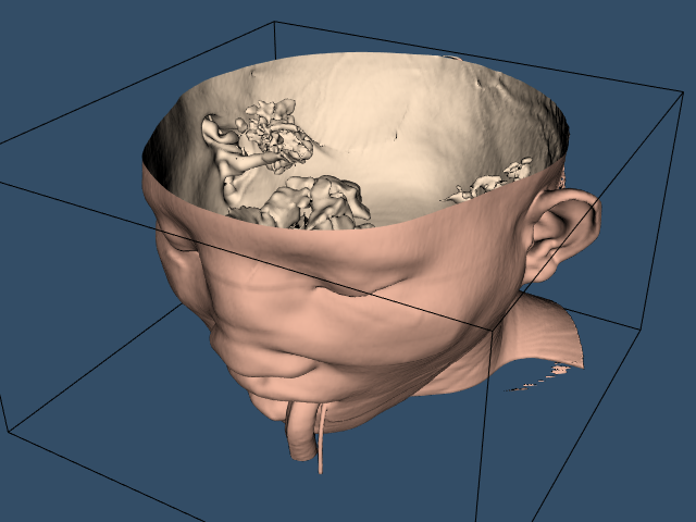 |
| Figure 12-3 | Skin and bone isosurfaces (Medical2.cxx). |  |
| Figure 12-4 | Composite image of three planes and translucent skin Medical3.cxx. | 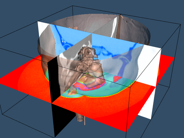 |
| Figure 12-6 | Photographic slice of frog (upper left), segmented frog (upper right) and composite of photo and segmentation (bottom). The purple color represents the stomach and the kidneys are yellow (frogSlice.tcl). | 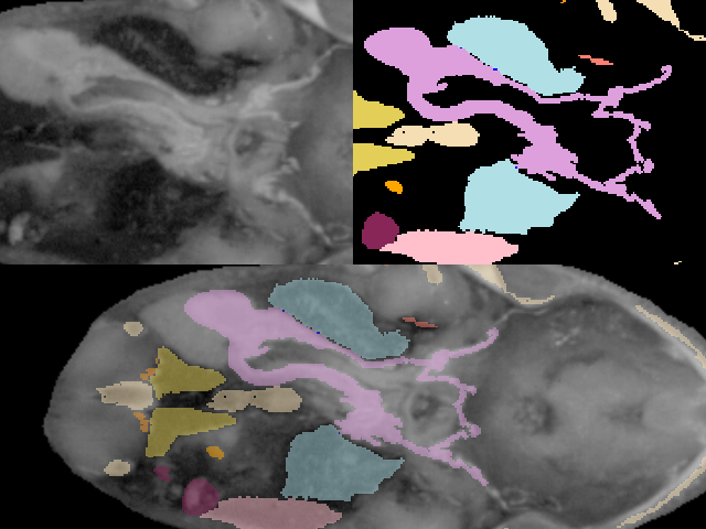 |
| Figure 12-7 | The frog’s brain. Model extracted without smoothing (left) and with smoothing (right). |  |
| Figure 12-9a-d | All frog parts and translucent skin. This script generates all four images. | 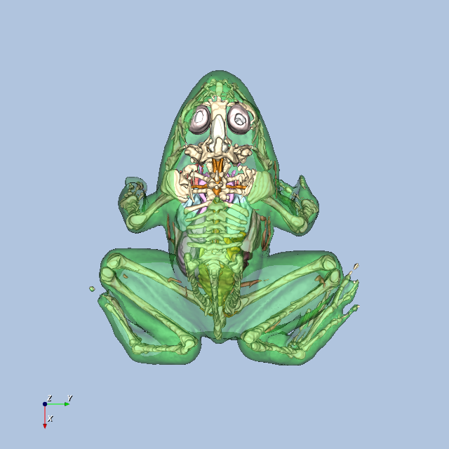 |
| Figure 12-11 | Two views from the stock visualization script. The top shows closing price over time; the bottom shows volume over time (stocks.tcl). |  |
| Figure 12-13 | A logo created with vtkImplicitModeller (vtkLogo.cxx). |  |
| Figure 12-14 | Portion of computational grid for the LOx post (LOxGrid.tcl). | 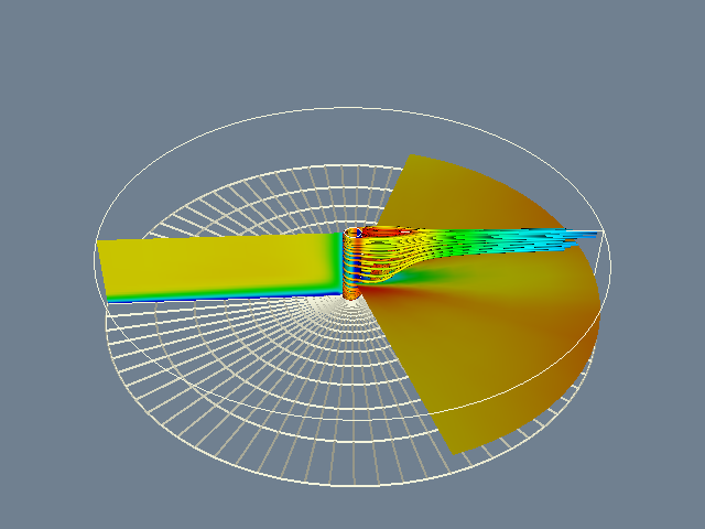 |
| Figure 12-15 | Streamlines seeded with spherical cloud of points. Four separate cloud positions are shown. | 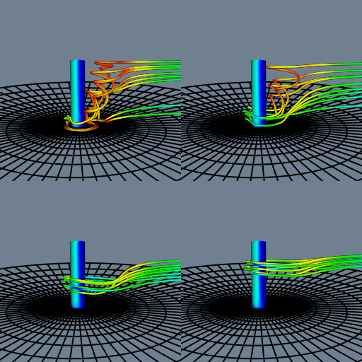 |
| Figure 12-16 | Streamtubes created by using the computational grid just in front of the post as a source for seeds (LOx.tcl). |  |
| Figure 12-17 | Ten frames from a blow molding finite element analysis. Mold halves (shown in wireframe) are closed around a parison as the parison is inflated. Coloring indicates thickness—red areas are thinner than blue (blow.tcl) | 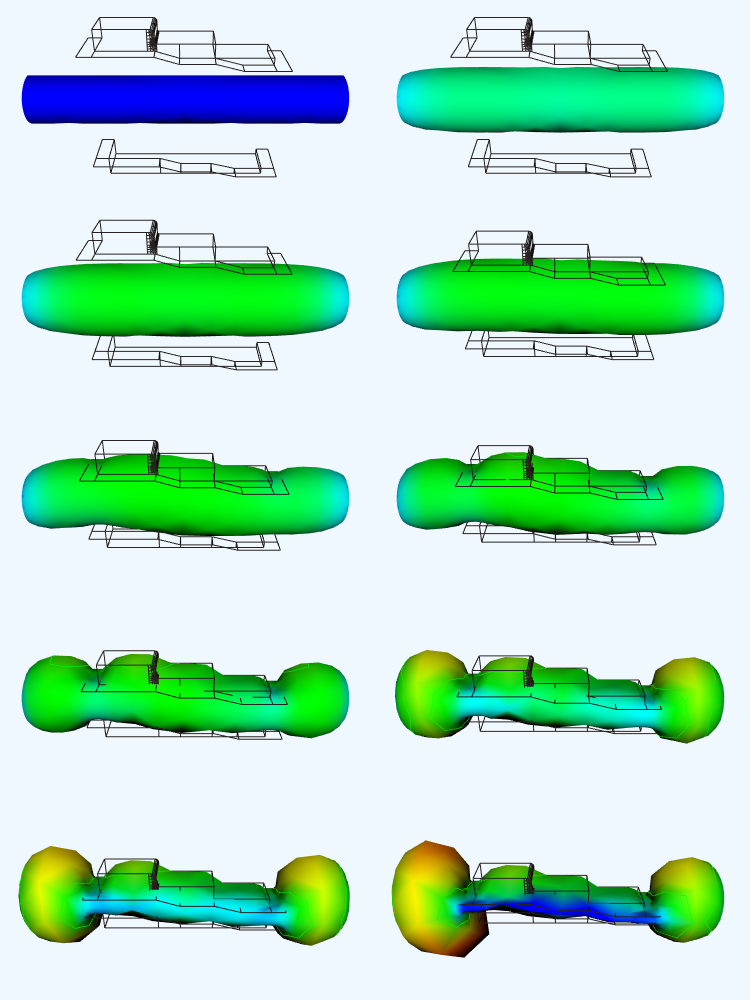 |
| Figure 12-20a | Towers of Hanoi. (a) Initial configuration. |  |
| Figure 12-20b | Towers of Hanoi. (b) Intermediate configuration. |  |
| Figure 12-20c | Towers of Hanoi. (c) Final configuration Hanoi.cxx. | 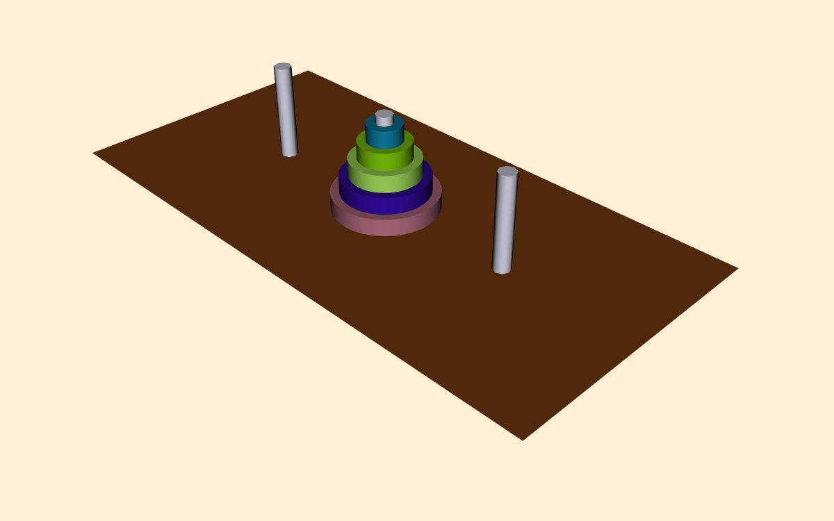 |