Fields, spaces and implicit arrays

A field's space determines which values can disagree and how to evaluate them inside a cell. Moving between spaces changes that interpretation. It can introduce averaging even when the geometry and topology remain the same. Start with Function Spaces and Degrees of Freedom for the meaning of H1, H2, L2 and polynomial order. This chapter applies those ideas to Tack's field and array representations.

For construction recipes, jump to L2 fields or quadratic H1 fields. Both use the same mesh and have runnable examples below.

Choose where values live

Space	Ownership	Use it for
td.H1(data, order=1)	One shared value per corner vertex	A continuous first-order nodal temperature or velocity
td.H1(data, order=2)	Shared corner, edge and supported face/interior nodes	A higher-order H1 approximation; not an H2 space
td.Constant(data)	One value per cell	Cell averages, material parameters
td.L2(data)	Each cell's own corner values	Discontinuous solution fields
td.Values(data, "faces")	One value per face, without an interpolation basis	Face areas, labels or fluxes
td.Values(data, "points" / "cells" / "edges")	One value per named entity kind	Entity attributes that need no basis
td.SideTraces(data)	Values per face, per side, per face corner	Two-sided evaluation, by projecting into it

For L2(order=0) the value is constant per cell; L2(order=1) uses each cell's own corners. H1(order=2) adds higher-order degrees of freedom on supported shapes. Values describes association without promising any interpolation between entities.

tack.empty((field.space.size,), tack.vec3()) allocates one 3-vector per DOF; td.Field(field.space, values) gives those values their mesh meaning. The array has shape (field.space.size,) and downloads as (field.space.size, 3).

The field's coefficient count is field.space.size. It agrees with data.num_points for H1 order 1, but not generally for other spaces. A vector field has one vector per space DOF, so the scalar component storage has that count times the vector width.

Constant means a separate constant function in each cell. ConstantArray means an array with one repeated value, regardless of space. These two independent choices can be combined: an H1 field with a ConstantArray is a spatially constant H1 function, while a Constant field backed by an ordinary array can assign different values to every cell.

Spaces belong to a topology and are interned there: repeated td.H1(data) uses the same layout. A field with a matching length on another topology is still a different association. Wrap values with the correct space when they are created; do not repair an association by guessing from array length later.

Construct an L2 field

The complete independent-spaces example builds L2 pressure and quadratic H1 temperature on the same two hexes. This section constructs pressure directly; the next section constructs temperature. The snippets assume NumPy, Tack and tack.dataset imported as np, tack and td, with a default device set.

Use uniform_grid as a shortcut for the mesh setup here; Build Meshes shows its explicit topology and geometry construction:

    # Shortcut mesh setup: two adjacent hexes in the unit cube.
    data = td.uniform_grid((3, 2, 2), spacing=(0.5, 1.0, 1.0))

Each hex has eight corners. td.L2(data, order=1) assigns a separate value to each of them: 16 coefficients, even though the topology has only 12 vertices. The four corners on the shared face each have two pressure coefficients. They occupy the same physical positions and may have different values. See the node-sharing diagram.

Initialize each cell's coefficients

Construct pressure as p = x in cell 0 and p = x + 2 in cell 1. It varies inside both cells and has a jump of 2 at x = 0.5. An L2 field need not be constant inside a cell.

The space supplies offsets: coefficient j of cell c is stored at offsets[c] + j. For these two hexes, the offsets are [0, 8, 16]:

Cell	Storage slots	Meaning
0	0 through 7	Its own corner values, in the cell's local corner order
1	8 through 15	Its own corner values, including its side of the shared face

The initialization kernel walks each cell's corners and writes its block. Every coefficient has one writer. Using offsets also works when cells have different corner counts; multiplying the cell id by eight would not.

@tack.kernel
def initialize_pressure(cells, offsets, values):
    for c in cells:
        cell_id = cells.entity_id(c)
        first = offsets[cell_id]
        for j in range(cells.NUM_POINTS):
            x = cells.corner_position(c, j)
            values[first + j] = x.x + 2.0 * cell_id

Allocate the values and attach their space:

    pressure_space = td.L2(data, order=1)
    pressure = tack.empty((pressure_space.size,))
    td.for_each(initialize_pressure, data, "cells", pressure_space.offsets, pressure)
    data.fields["pressure"] = td.Field(pressure_space, pressure)

td.for_each supplies the geometry-aware cell view, so corner_position returns physical coordinates. The resulting Field contains the original cell-local coefficients; no shared-point averaging is involved.

Copy coefficients from an existing solver array

If you already have nodal DG coefficients in this order, upload them directly. For this particular pair of hexes, this constructs the same pressure field:

    # Each row follows that hex's local corner order: 0, 1, ..., 7.
    per_cell = np.array([
        [0.0, 0.5, 0.5, 0.0, 0.0, 0.5, 0.5, 0.0],   # cell 0: p = x
        [2.5, 3.0, 3.0, 2.5, 2.5, 3.0, 3.0, 2.5],   # cell 1: p = x + 2
    ], dtype=np.float32)
    uploaded_pressure = td.Field(pressure_space, tack.array(per_cell.reshape(-1)))

The two eight-value rows describe the cells' local nodes, not eight globally unique points each. Flattening these rows preserves both interface values. For a mixed-cell mesh, use pressure_space.offsets and the appropriate local corner order to assemble the blocks; a rectangular (num_cells, 8) array is specific to the all-hex example. Coefficients in another basis need conversion before this upload, as in MFEM import.

A constant inside each cell: L2 order 0

Choose order 0 for one independent coefficient per cell:

    cell_space = td.L2(data, order=0)
    cell_pressure = td.Field(cell_space, tack.array([1.0, 3.0], dtype=tack.f32))

Here cell_space.size is two. Values 1 and 3 are constant inside their own cells and differ across the interface. td.Constant(data) is another representation of that piecewise-constant function meaning; it also supports topologies without reference elements.

Evaluate and check the discontinuity

    pressure_centers = td.values_at_centers(data, "pressure")
    pressure_gradient = td.gradients(data, "pressure")
    pressure_jump = td.jump(data, "pressure")
    # Centers: [0.25, 2.75]; gradients: [1, 0, 0]; interface jump magnitude: 2.

For the varying order-1 pressure, the cell centers hold [0.25, 2.75] and both physical gradients are [1, 0, 0]. The one interior face has jump magnitude 2; jump's sign follows its side ordering. The runnable check compares the uploaded coefficients with the kernel-initialized ones as well. These are cell-interior gradients; the interface discontinuity is represented separately by the jump.

Construct a quadratic H1 field

On the same mesh, construct T = x² + 2y + 3z using td.H1(data, order=2). The geometry stays first-order H1 and still has 12 corner positions. Temperature has 45 global nodal coefficients, including nodes away from corners.

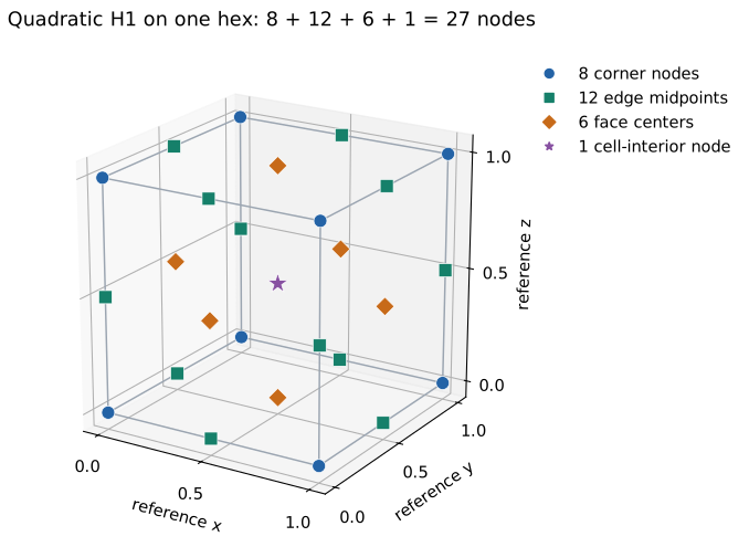
A single quadratic hex uses three nodes per reference coordinate direction: the tensor-product layout has 3 × 3 × 3 = 27 nodes. Two adjacent hexes share nine on their common face: its four corners, four edge midpoints and face center. Thus 27 + 27 - 9 = 45 global DOFs. Count the two-cell mesh by entity as follows:

Location	Global temperature DOFs
Topological corner vertices	12
Edge midpoints	20
Face centers	11
Cell interiors	2
Total	45

These are field nodes on the original two cells. They do not subdivide the mesh, change corner connectivity, or make its geometry quadratic.

Sample at the field's nodes

First define the function to sample:

@tack.func
def quadratic_temperature(x):
    return x.x * x.x + 2.0 * x.y + 3.0 * x.z

interpolate evaluates it at every node of the temperature space, where the geometry puts each one, and returns the field:

    temperature_space = td.H1(data, order=2)
    # The function at all 45 temperature nodes, not just the 12 corners.
    data.fields["temperature"] = td.interpolate(data, quadratic_temperature,
                                                temperature_space)

The space builds local-to-global addressing for shared corners, edges and faces. Its node numbering is not simply 27 consecutive entries per cell. interpolate writes a shared node once, from the first cell that has it, rather than from every adjacent cell, and stores no node positions: each is evaluated through the geometry as it is needed. To see where the nodes are, project the geometry into the space (td.project(data, data.geometry, temperature_space)); that does not change data.geometry.

Interpolating differs from projecting a first-order solution into a quadratic space: that conversion retains the original first-order function. To represent this quadratic, interpolate it as above, or supply the original quadratic coefficients in Tack's nodal basis and ordering.

Evaluate through the quadratic basis

    at_centers = td.values_at_centers(data, "temperature")
    gradient = td.gradients(data, "temperature")
    linearized = td.project(data, "temperature", td.H1(data, order=1))
    linear_centers = td.values_at_centers(data, linearized)

At the two cell centers, quadratic evaluation gives [2.5625, 3.0625] and physical gradients [0.5, 2, 3] and [1.5, 2, 3]. Projecting this temperature down to H1 order 1 gives center values [2.625, 3.125]. The latter keeps the corner values but changes the function between them.

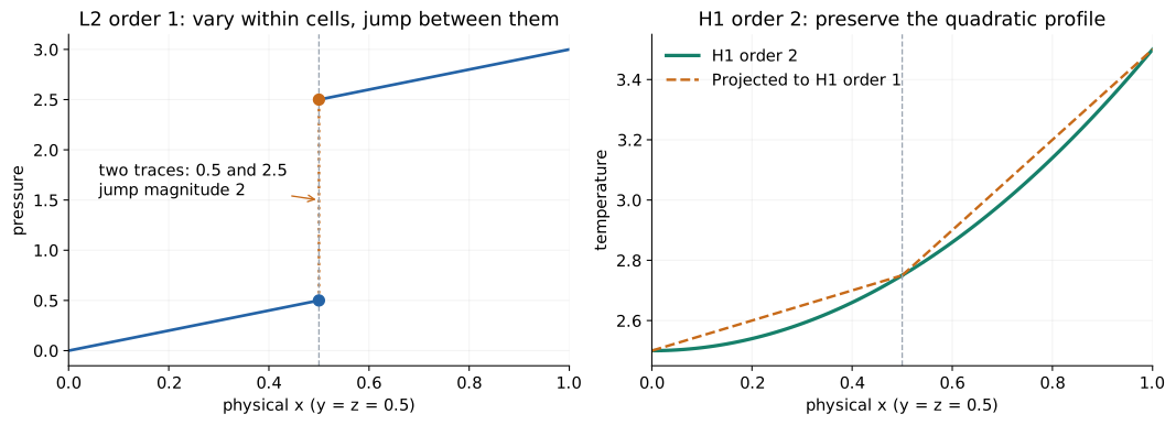
Both profiles are evaluated through the fields' actual bases along y = z = 0.5, including the two separate L2 traces at x = 0.5. The dotted vertical pressure segment marks the jump, not an interpolated connection. The geometry and topology are identical for every curve. Quadratic H1 enforces shared values; it does not generally enforce matching derivatives or H² conformity.

Run the complete program and reproduce all three diagrams:

uv run python docs/examples/data_spaces.py --check
uv run --with matplotlib python docs/examples/data_spaces.py --check --figures /tmp/tack-space-figures

The optional plotting step writes standalone SVG and PNG files. The numerical checks run without Matplotlib.

A material interface exposes the difference

The two-cell example has material 1 on the left and 3 on the right. Converting it to shared point data gives value 2 on the common face. Converting it to L2 preserves both sides of the discontinuity:

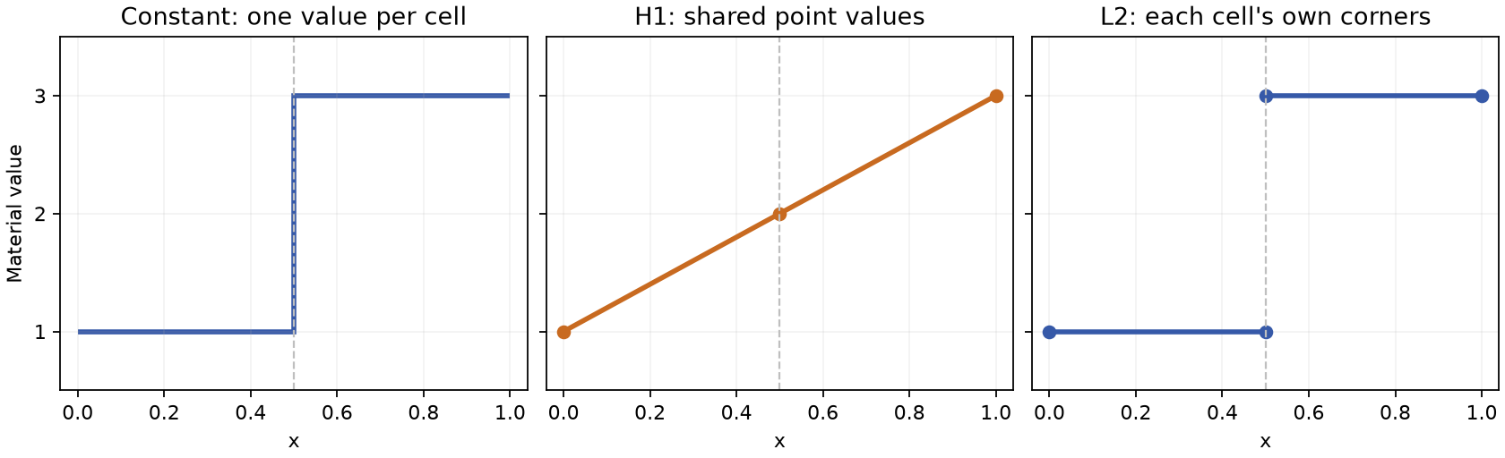
The figure is generated from the example's values along the bottom front edge; the dashed line is the shared face at x = 0.5. The middle ramp is an effect of projection and interpolation, not an interface resolved by the original data. H1 and L2 both use order 1 in this figure.

    cell_temperature = td.project(data, "temperature", td.Constant(data))
    point_material = td.project(data, "material", td.H1(data))
    separate_material = td.project(data, "material", td.L2(data))
    gradient = td.gradients(data, "temperature")

The returned objects are fields. Assign one to data.fields[name] if later filters should carry it. Computing point_material alone does not add it to the dataset's named fields.

Projection is an algorithmic choice

project(data, field, target_space) is the one operation: td.H1(data), td.Constant(data) and td.L2(data) are the common target spaces.

Conversion	Meaning	What to check
H1 → Constant	Mean of each cell's corner values	Not a general volume integral
Constant → H1	Mean of incident cell values at each point	Material discontinuities become shared values
H1 → L2 of sufficient order	Evaluate the continuous field at each cell's local nodes	Values remain equal on shared interfaces
L2 → H1	Evaluate from adjacent cells, then average	Jumps can be smoothed
Constant → L2(order=1)	Repeat a cell's value at its own corners	Discontinuities remain

For the affine temperature x + 2y + 3z on the two regular cells, corner means are [2.75, 3.25], the exact center values. That convenient property does not establish conservation for general fields or distorted cells.

Polyhedral, polygonal and polyline topologies support point/cell projection. L2, higher-order projection and traces require the shape-based path. In particular, being able to attach point values to a polyhedron does not imply that it supplies shape-function evaluation for every algorithm.

Read both sides of a face

    face_values = td.project(data, "material", td.SideTraces(data))
    material_jump = td.jump(data, "material")
    continuous_jump = td.jump(data, "temperature")

Projecting into SideTraces evaluates each cell at its faces' corners, keeping the two sides separate and aligned in the face's ordering. jump evaluates a difference at each face center: side 1 minus side 0, or zero at a boundary.

The material has one nonzero jump of magnitude 2. The affine H1 temperature has zero jump. The sign of a material jump depends on the face's side ordering; its magnitude does not. A face normal points out of side 0. These conventions matter when assembling a flux and are developed in Mesh Kernels.

For a normal-oriented face quantity, use Values(data, "faces", oriented=True). A filter that reverses a carried face then negates the value. Area and labels are ordinary, unoriented face values and should not change sign.

Values can be computed instead of stored

Uniform-grid coordinates need only dimensions, origin and spacing; allocating three scalars for every point would be redundant. An implicit value array provides a get(k) expression that Tack inlines into the consuming kernel.

Geometry's space and its implicit array are different layers

Both an image and a rectilinear grid have an order-1 H1 geometry field. Its space says how a cell's nodal positions define a coordinate mapping; its implicit value array says how to obtain each nodal position. The two layers can change independently:

Geometry values	Information retained	How one nodal position is obtained
UniformCoordinates	Dimensions, origin, spacing and direction	Evaluate the uniform-grid coordinate formula
CartesianProduct	Three backend axis arrays	Gather one coordinate from each axis
Explicit tack.Array with dtype tack.vec3(...)	One stored 3-vector per geometry DOF	Read the vector

Calling materialize on image coordinates changes their storage into an explicit value array; it does not change H1 order, add cells, or turn StructuredTopology into UnstructuredTopology. Calling to_host creates a host snapshot without replacing the geometry's value representation. See the geometry formulas and topology combinations.

Do not infer a function space from an array class. A CartesianProduct describes a way to compute 3-vectors; H1 describes how coefficients are associated and interpolated on a topology. td.Field couples these two choices, with a check that the value count matches the space.

Other implicit coefficient arrays

    data.fields["constant"] = td.Field(td.H1(data), tack.arrays.ConstantArray(5.0, data.num_points))
    explicit = tack.arrays.materialize(data.fields["constant"].values)
    snapshot = tack.arrays.to_host(data.fields["constant"].values)

Here ConstantArray stores the constant and count, not 12 separate values. materialize computes storage on the default device. to_host evaluates and downloads a snapshot. Neither changes the original field's representation.

Implicit array	Useful when
UniformCoordinates, CartesianProduct	Coordinates follow a uniform or rectilinear grid
ConstantArray, CountingArray	Values are constant or a sequence
Permutation, View, Strided	Values are selected or reorganized without a new value buffer
ExtractComponent, Components	Scalar components and vector values need to be connected
Transform, Function, Cast	A device function or conversion can compute values on demand

Operands can themselves be implicit arrays. This keeps intermediates out of storage, but the expression still does work whenever it is read. Materialize an expensive expression if reuse makes that worthwhile, then measure the whole pipeline. An implicit wrapper around a mutable buffer observes its current values; a materialized result is a previous computation until recomputed.

Know the present higher-order limits

Order-2 H1 is supported on tetrahedra, hexahedra, voxels and wedges, and on their faces' shapes: triangles, quads and pixels. L2 can vary its order by cell, which the dispatcher handles by launching groups of compatible order. This does not make every filter a higher-order geometric algorithm: extract_surface keeps a solid's order-2 fields and geometry at order 2 (its surface's nodes are the solid's), but other extractions carry corner values, and higher-order subdivision remains open work. The reference records the supported layouts and filter propagation rules.

Run and reproduce the figure

uv run python docs/examples/data_fields.py --check
uv run --with matplotlib python docs/examples/data_fields.py --check --output spaces.png

Download the complete program. Continue with Filtering and Analysis.