Filter and analyze datasets¶

Choose a filter by what should happen to the cells. Keeping a whole cell, cutting a cell, and extracting its intersection with a surface answer different questions, even when all three use the same scalar threshold.

The running example samples x and the velocity [-y, x, 0] on a grid covering [-1, 1]³. The simple analytic fields make the results independently checkable.

Prepare named inputs¶

@tack.kernel
def sample(xyz, scalar, velocity):
    for p in range(scalar.shape[0]):
        x = xyz.get(p)
        scalar[p] = x.x
        velocity[p] = [-x.y, x.x, 0.0]

    data = td.uniform_grid((9, 5, 5), origin=(-1, -1, -1), spacing=(0.25, 0.5, 0.5))
    x = tack.empty((data.num_points,))
    velocity = tack.empty((data.num_points,), tack.vec3(tack.f32))
    sample(data.geometry.values, x, velocity)
    data.fields["x"] = td.Field(td.H1(data), x)
    data.fields["velocity"] = td.Field(td.H1(data), velocity)

The complete script supplies the imports and initializes the backend. All following fragments use this dataset. A field argument can be its name or the td.Field itself; a raw value buffer needs a space wrapper first.

Select cells, cut cells, or extract a surface¶

Goal	Operation	Output
Keep cells whose scalar lies in an interval	`threshold`	Whole cells, preserving their shapes
Keep cells inside a region described by a function	`extract_geometry`	Whole cells
Keep a named or explicit cell selection	`extract_cells`	Whole cells in input order
Keep a box of a structured grid, every n-th point	`extract_extent`	A structured grid of the same kind (VTK's `vtkExtractGrid`/`vtkExtractVOI`); a one-point-thick box is a grid of one dimension less
Normals of a surface, its polygons wound alike	`surface_normals`	The surface with `normals` on points and `cell_normals` on cells (VTK's `vtkPolyDataNormals` without splitting)
Keep the part on one side of a level	`clip`	Whole cells and pieces of cut cells
Extract a scalar level set, or several	`contour`	Triangles in 3D; line cells in 2D; vertices on lines; `dimension=` picks which cells of a mixed mesh (the highest by default, never mixed); with several values, all of them, each cell's in `contour_value`
Intersect with a plane or another implicit function, or several parallel ones	`slice_plane`, `slice`	Intersection geometry
Keep original points by scalar or region	`threshold_points`, `extract_points`	Vertex cells, without cell connectivity

For point data, threshold checks every corner by default. With all_points=False, one in-range corner suffices. Neither option interpolates a cut boundary. For cell data, the cell's one value makes the selection.

    whole = td.threshold(data, "x", 0.125, 1.0)                  # all corners in range
    touching = td.threshold(data, "x", 0.125, 1.0, all_points=False)
    plane = td.Plane(origin=(0.125, 0, 0), normal=(1, 0, 0))
    clipped = td.clip(data, plane, fields=["x"])                # keep x >= 0.125
    surface = td.contour(data, "x", 0.125, fields=["velocity"])
    section = td.slice_plane(data, origin=(0.125, 0, 0), normal=(1, 0, 0))

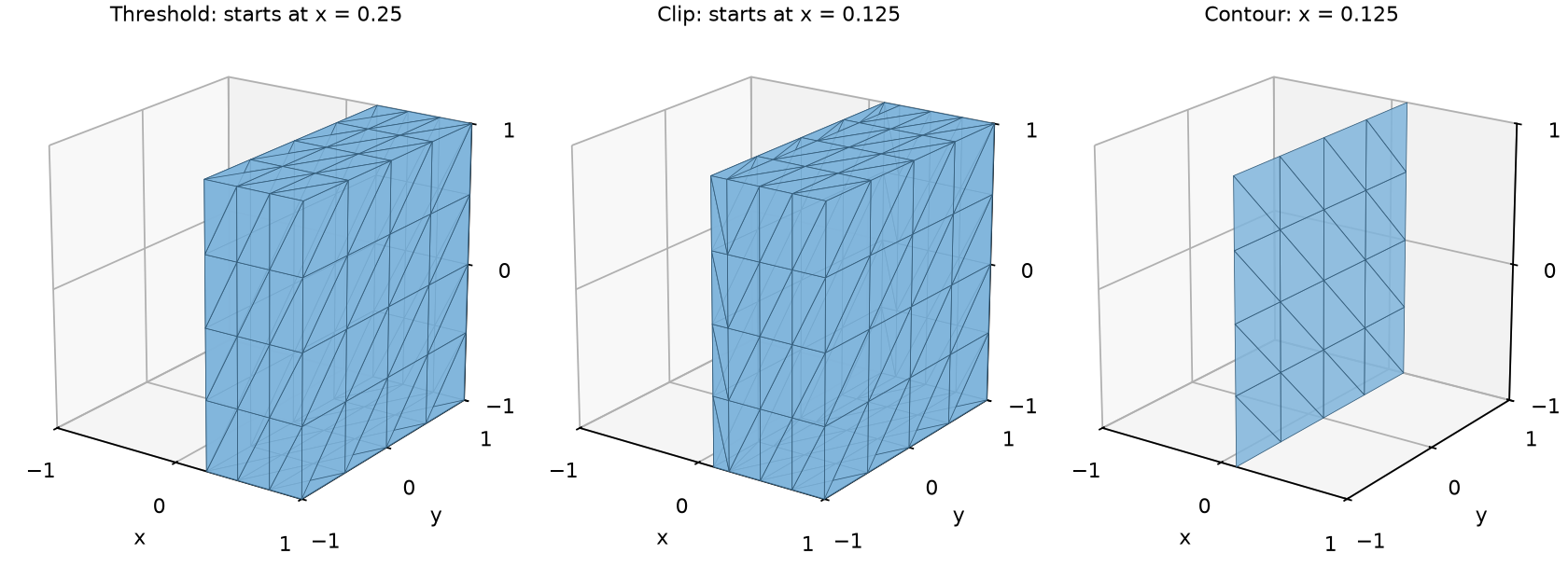
Whole-cell selection, clipped cells, and an extracted level set

At x = 0.125, no grid plane coincides with the requested boundary. The threshold keeps 48 cells starting at x = 0.25, with total volume 3. The clipped region starts at x = 0.125 and has volume 3.5. The contour is a plane of area 4. all_points=False keeps 64 whole cells, including a layer that crosses the threshold. These different measures are intentional.

Understand the sign of an implicit function¶

Plane, Sphere, Cylinder, Box and Planes expose a value(position) that is negative inside, zero on the boundary and positive outside. For the plane in the example it is x - 0.125. Union, Intersection and Difference combine them (Difference(box, sphere) is the box with a ball taken out), as VTK's vtkImplicitBoolean does, on the device.

clip(data, plane) keeps values at or above zero, here the positive-x side. Pass inside=True to keep the other side, inside the function's region. extract_geometry instead defaults to inside=True, the negative side, and keeps whole cells. State which region you mean before choosing flags; the words “inside” and “keep” do not by themselves specify the same default for both functions.

Decide which fields follow the geometry¶

Filters creating datasets accept fields=: all named fields by default, a name or list to select them, and [] for geometry alone. Geometry is always handled separately. An unknown requested name raises KeyError.

Input association	Typical propagation
Floating point data	Gathered for kept points; interpolated onto edge crossings
Cell data	Copied to each retained cell or each piece of an input cell
L2 data	Retained cell by cell when whole cells survive on a shape-based output
Face values	Retained only when the filter has a face map; on an extracted surface, mapped to output cells where supported
Side traces or entities with no propagation map	Left behind

For example, the contour above carries only velocity, interpolated at its new points; the clip carries only x. Computing a derived field does not automatically name it: put it in data.fields before extraction if it should travel with the result.

Integer point labels are not interpolated as continuous data. Use cell labels when that is the intended association. To preserve provenance of cell pieces, attach td.cell_ids(data) as a named cell field before filtering; its ids then refer to the source mesh, while output cell ids refer to the new mesh.

Sets follow provenance, not geometric guesses¶

Cell sets survive selections and follow pieces of selected cells. A face set can become a cell set when its faces become surface cells. Newly generated points do not automatically inherit a point set merely because they lie near an old selected point. The result follows the filter's entity maps.

The mixed-mesh example names a roof cell and a boundary face set, then filters:

    mesh.sets["boundary"] = td.boundary_faces(mesh)  # a face Set
    mesh.sets["roof"] = td.Set(mesh, "cells", [1])   # a cell Set
    kept = td.threshold(mesh, "material", 1.5, 3.0)  # sets come along
    print(f"boundary: {len(mesh.sets['boundary'])} faces; the roof is cell "
          f"{kept.sets['roof'].numpy()} of the threshold")

Its returned roof id is zero after thresholding because the output cells have been renumbered. Use the returned set with the returned dataset.

Derived fields and summaries¶

    speed = td.magnitude(data, "velocity")
    data.fields["speed"] = speed                               # keep the returned field
    velocity_gradient = td.gradients(data, "velocity")
    flow = td.flow_quantities(data, velocity_gradient)
    summary = td.statistics(data, "x")

magnitude returns a field in the velocity's space. gradients returns cell gradients by default; at="points" evaluates and averages onto points. For a 3-vector field its gradient has nine components, in row order d(u_i)/d(x_j). flow_quantities derives divergence, vorticity and Q from it. The solid rotation in this example has divergence 0, vorticity [0, 0, 2] and Q = 1 in every cell.

statistics summarizes stored field samples, not a volume integral. An arithmetic mean of point temperatures is not a volume-weighted mean on a stretched mesh. Choose cell measures and a suitable quadrature when the quantity you need is a physical integral. The function returns Python values and therefore waits for the device work it reads.

Cell quality¶

cell_quality(data, measures) measures how well shaped each cell is, a cell field per measure, each 1 on the ideal cell of its shape (equilateral; a cube, a regular tetrahedron):

Measure	What it says
`scaled_jacobian`	the worst corner's edges' determinant, edges scaled to unit length, relative to the ideal cell's: 1 ideal, 0 flat, negative inverted
`jacobian_ratio`	the least corner determinant over the greatest: 1 for every simplex, below 1 as a cell tapers
`condition`	the worst corner's condition number against the ideal cell's: 1 ideal, growing as it distorts, the largest float when inverted
`edge_ratio`, `min_edge`, `max_edge`	the longest edge over the shortest; the shortest and longest, in the spatial unit

They are Verdict's definitions (VTK's vtkMeshQuality), matched to VTK where it defines them, and extended to every shape Tack has: the corners' edges are the geometry's Jacobian applied to the reference cell's edge directions, so order-2 cells are measured along their curved edges, and wedges and pyramids get every measure. Polyhedra and polygons, which have no reference cell, are measured by the fan tetrahedra and triangles Tack evaluates them in.

import numpy as np

import tack
import tack.dataset as td

tack.set_default_device("cpu")

mesh = td.tetrahedralize(td.uniform_grid((4, 4, 4)))
quality = td.cell_quality(mesh, ["scaled_jacobian", "condition", "edge_ratio"])
sj = quality["scaled_jacobian"].values.numpy()
print(f"scaled Jacobian {sj.min():.3f} to {sj.max():.3f}")
mesh.fields["sj"] = quality["scaled_jacobian"]
worst = td.threshold(mesh, "sj", -1.0, 0.75)          # the right-corner tetrahedra
assert np.isclose(sj.max(), 1.0) and np.isclose(sj.min(), 1 / np.sqrt(2))
assert worst.num_cells == np.count_nonzero(sj < 0.75)

Feature edges¶

feature_edges(data, angle=30.0) finds a surface's edges by how many cells meet there and at what angle, as VTK's vtkFeatureEdges: boundary edges (one cell), feature edges (two cells whose normals are at least angle degrees apart), non-manifold edges (three or more cells) and, if asked, manifold edges (the rest of the two-cell edges). The result is line cells on the same points with a kind cell field (EdgeKind), point fields carried. A volume mesh's surface comes from extract_surface first.

import numpy as np

import tack
import tack.dataset as td

tack.set_default_device("cpu")

box = td.uniform_grid((4, 3, 3))
surface = td.extract_surface(box, td.boundary_faces(box))
edges = td.feature_edges(surface)                 # the box's 12 edges, in segments
kinds = edges.fields["kind"].values.numpy()
print(edges.num_cells, "feature edges")
assert (kinds == td.EdgeKind.FEATURE).all() and edges.num_cells == 4 * 3 + 4 * 2 + 4 * 2
open_top = td.uniform_grid((4, 4))
assert td.feature_edges(open_top).num_cells == 12           # its boundary

Check algorithm support before building a pipeline¶

Task	Shape-based	Polyhedral / polygonal	Polyline
Select whole cells; measure cells	Yes	Yes	Yes
Extract boundaries	Yes, subject to line-cell limitations	Yes	Chain ends
Contour or slice	Yes, of order-1 and `L2` fields (an order-2 `H1` field is refused)	Yes	Contour: vertices, of point data
Clip cells	H1 geometry required	Polyhedra: yes, into polyhedra (faces clipped, iso-polygons as caps); polygons not yet	Currently unsupported
Project between point and cell data	Yes	Yes	Yes
Gradients and flow quantities	Yes (2D cells in their plane)	Yes: Green–Gauss over each polyhedron's faces, and over each polygon's edges in its plane (exact for linear fields)	Yes (zero)
Locate cells and probe	Yes	Yes: in sub-tetrahedra or fanned triangles; cells must be star-shaped from their points' mean	Yes, on segments
Advection and streamlines	Yes, 2D and 3D cells	Yes, as probing locates	Currently unsupported
Carry ghost marks over pieces	Yes	Yes	Yes

An empty supported filter result is a valid dataset. Check num_cells before assuming an extraction contains visible geometry. Algorithms requiring a reference element reject unsupported topologies; storing H1 values alone does not change that support. The reference matrix has the details.

Run and check¶

uv run python docs/examples/data_analysis.py --arch cpu --check
uv run --with matplotlib python docs/examples/data_analysis.py --check --output filters.png

The checks include counts, independently calculated volumes and areas, interpolated velocity, flow derivatives, probe validity and analytic rotation. Download the complete program.

Continue with Mesh Kernels to implement an operation, or Sample and Connect Simulations to connect stages.